Probability of unemployment
Unfortunately, our grant has run out, so we can only afford to sample 10 people:
Data:
We’ll use this data to estimate the probability of unemployment in two ways
Probability of unemployment
Maximimum-likelihood (frequentist) estimation:
- Pick an estimator (such as sample proportion) of the probability
- Generate a point estimate of
- Use an approximation of the sampling distribution to quantify uncertainty:
- Generate a confidence interval (e.g.
Probability of unemployment
Posterior (Bayesian) estimation:
- Pick a prior (such as a uniform distribution) for the probability
Probability of unemployment
Posterior (Bayesian) estimation:
- Pick a prior (such as a uniform distribution) for the probability
- Update prior with data (one at a time or all at once)
(E)
Probability of unemployment
Posterior (Bayesian) estimation:
- Pick a prior (such as a uniform distribution) for the probability
- Update prior with data (one at a time or all at once)
(E, E)
Probability of unemployment
Posterior (Bayesian) estimation:
- Pick a prior (such as a uniform distribution) for the probability
- Update prior with data (one at a time or all at once)
(E, E, E)
Probability of unemployment
Posterior (Bayesian) estimation:
- Pick a prior (such as a uniform distribution) for the probability
- Update prior with data (one at a time or all at once)
(E, E, E, U)
Probability of unemployment
Posterior (Bayesian) estimation:
- Pick a prior (such as a uniform distribution) for the probability
- Update prior with data (one at a time or all at once)
(E, E, E, U, U)
Probability of unemployment
Posterior (Bayesian) estimation:
- Pick a prior (such as a uniform distribution) for the probability
- Update prior with data (one at a time or all at once)
(E, E, E, U, U, E, E, E, U, E)
Probability of unemployment
Posterior (Bayesian) estimation:
- Pick a prior (such as a uniform distribution) for the probability
- Update prior with data (one at a time or all at once)
- The posterior distribution describes the relative posterior probability for different values of
(E, E, E, U, U, E, E, E, U, E)
Comparing estimates
Maximum likelihood:
Posterior:
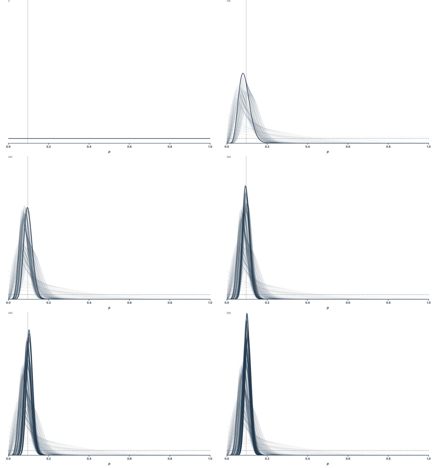
Bayesian updating
500 samples; uniform prior (click to animate)
Bayesian updating
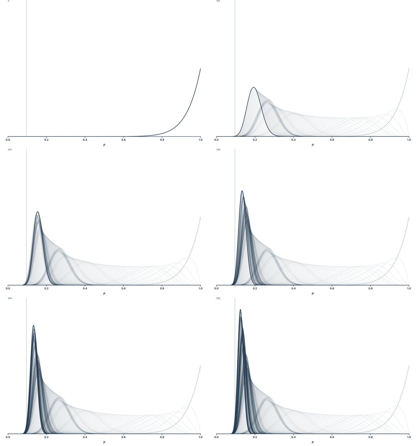
500 samples; “informative” prior (click to animate)
Conditional probability
The “posterior” is represented as a conditional probability distribution (the probability of varying values of
Bayes’ rule
Bayes’ rule is a simple formula that allows us to ‘flip’ a conditional probability
And for our unemployment model this becomes
Bayes’ rule
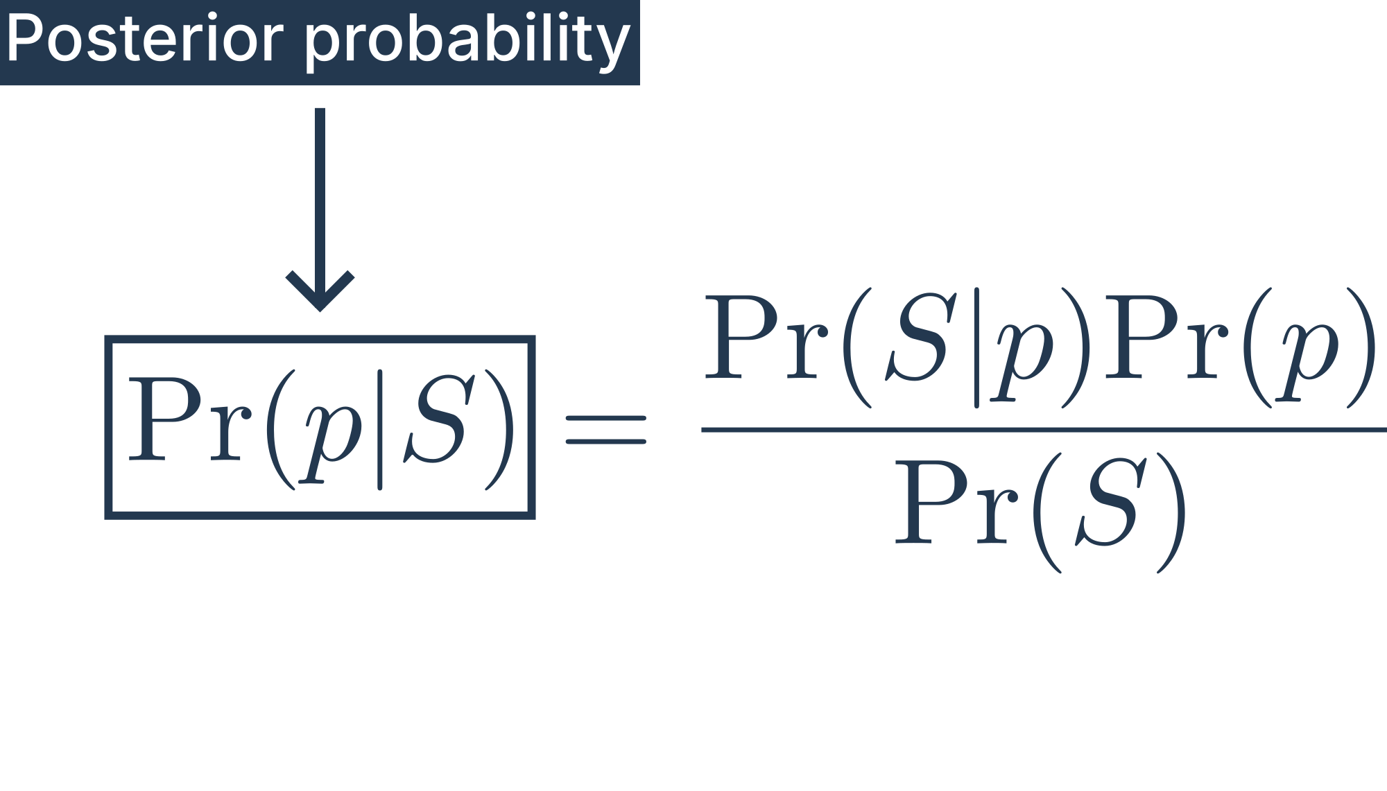
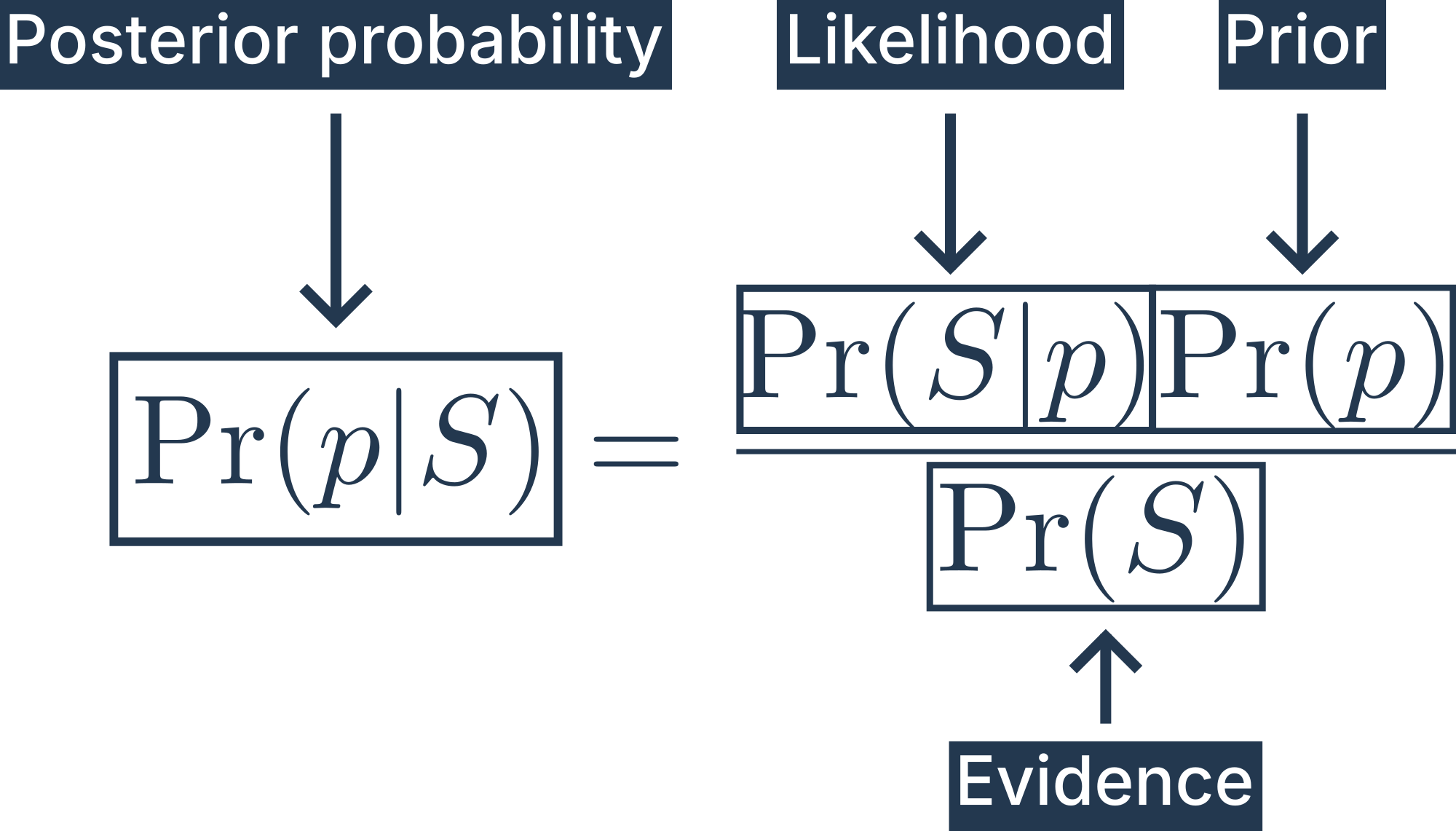
Posterior probability:
The posterior probability is our answer. It tells us everything we know about the probability of unemployment rate (
Bayes’ rule
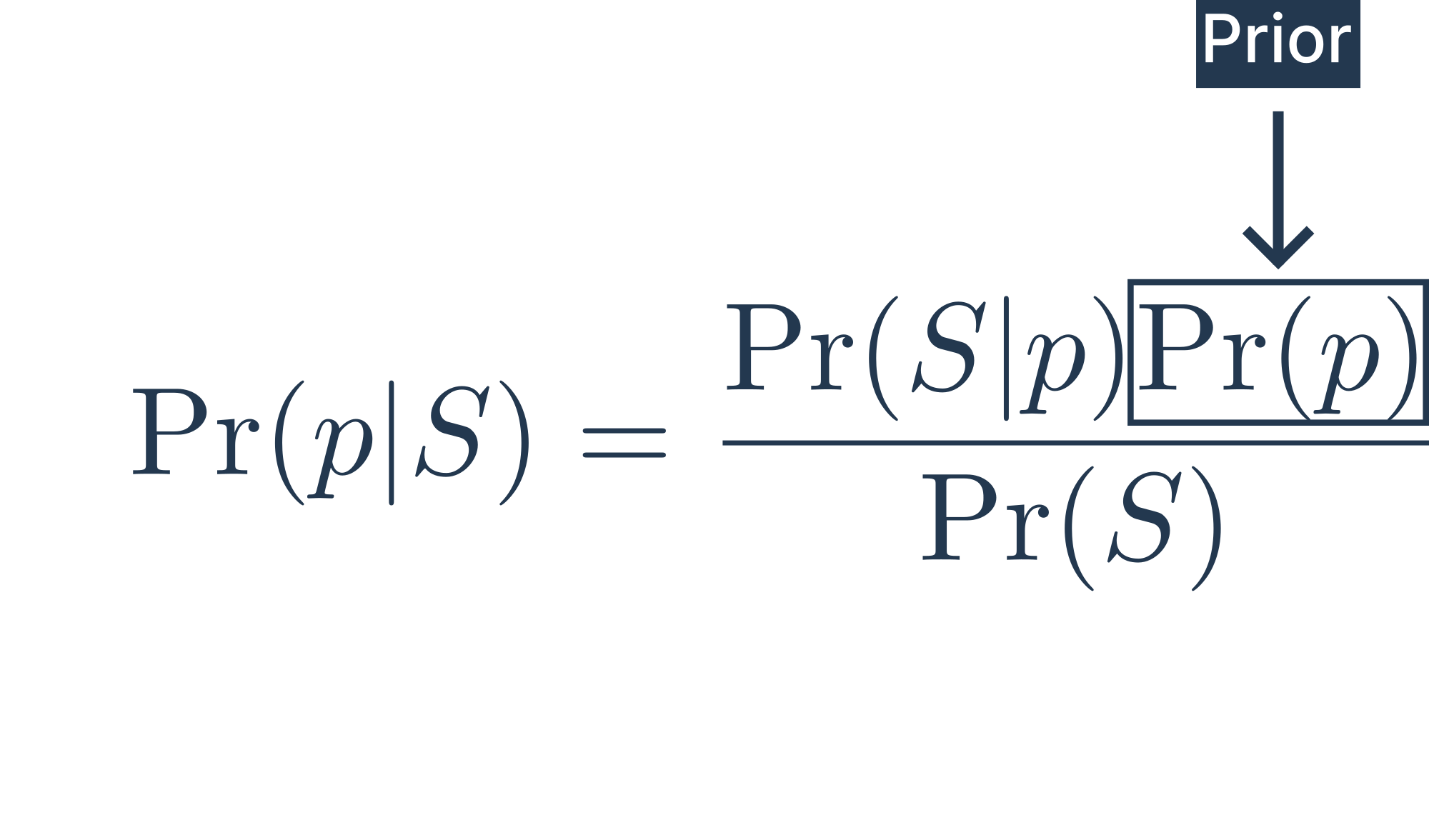
Prior probability:
The prior probability is everything we claim to know about the probability of unemployment (
Bayes’ rule
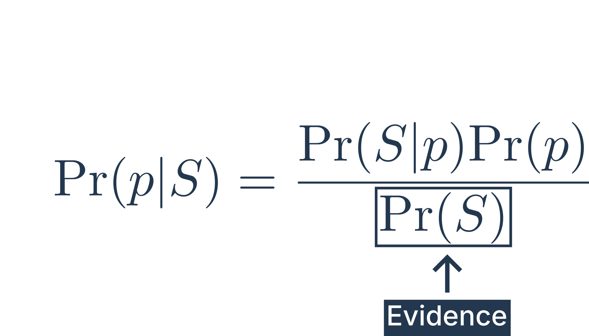
Evidence:
The evidence is just the average probability of seeing our sample across all possible values of
Fortunately we can almost always ignore it.
Bayes’ rule
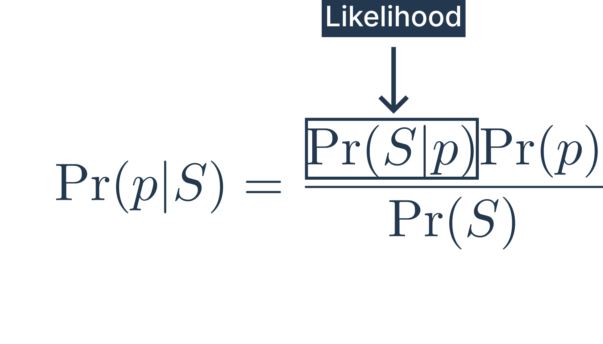
Likelihood:
The likelihood is where our model lives.
Building a parametric model
How to build a parametric model
- Pretend that we already know the probability of being unemployed (
- Tell a story about what our sample
Reverse the logic of your question
In reality we know
In our model we know
Building a parametric model
Binomial distribution
The probability of getting
Bayes’ rule
Likelihood:
The likelihood is where our model lives.
In this case, a binomial distribution is a good choice. Given a particular probabily of unemployment

Bayes’ rule
Proportional posterior
In practice, we rarely need to calculate the “evidence” (the denominator) in Bayes’ formula:
The posterior probability is proportional to (
Proportional posterior
Hands on: R and RMarkdown
Sample R script
- R scripts are plain-text files containing commands to be interpreted by R
- Example:
https://soci620.netlify.app/labs/handson_01_RvsRmarkdown.R
Sample RMarkdown document
- RMarkdown documents are plain-text files that mix regular text with R code.
- RMarkdown files can be ‘rendered’ to PDF, HTML, or MS Word files that are suitable for distribution.
- Example .Rmd file:
https://soci620.netlify.app/labs/handson_01_RvsRmarkdown.Rmd - Resulting HTML:
https://soci620.netlify.app/labs/handson_01_RvsRmarkdown.html
Image credit
Figures by Peter McMahan (source code)

Derrick Mercer, CC BY-SA 2.0, via Wikimedia Commons